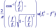
Tools |
||||||||||||||||||||||||||||||||||||||||||||||||||||||||||||||||||||||||||||||||||||||||||||||||
Certain
tools are central to the processing of digital images. These include
mathematical tools such as convolution, Fourier analysis,
and statistical descriptions, and manipulative tools such
as chain codes and run codes. We will
present these tools without any specific motivation. The motivation will
follow in later sections.
|
|
|
|
|
|
|
T.1
Rectangle |
|
|
|
|
|
picture 1 |
|
picture 2 |
|
|
|
|
|
|
T.2
Pyramid |
|
|
|
|
|
picture 1 |
|
picture 2 |
|
|
|
|
|
|
T.3
Pill Box |
|
|
|
|
|
picture 1 |
|
picture 2 |
|
|
|
|
|
|
T.4
Cone |
|
|
|
|
|
picture 1 |
|
picture 2 |
|
|
|
|
|
|
T.5
Airy PSF |
|
|
|
|
|
picture 1 |
|
picture 2 |
|
|
|
|
|
|
T.6
Gaussian |
|
|
|
|
|
picture 1 |
|
picture 2 |
|
|
|
|
|
|
T.7
Peak |
|
|
|
|
|
picture 1 |
|
picture 2 |
|
|
|
|
|
|
T.8
Exponential Decay
|
|
|
|
|
|
picture 1 |
|
picture 2 |
Table 4: 2D Images and their Fourier Transforms
Because of the monotonic, non-decreasing character of P(a) we have that:
![]()
For
an image with quantized (integer) brightness amplitudes, the
interpretation of
![]() a
is the width of a brightness interval. We assume constant width
intervals. The brightness probability density function is
frequently estimated by counting the number of times that each
brightness occurs in the region to generate a histogram, h[a].
The histogram can then be normalized so that the total area under the
histogram is 1 (eq. ). Said another way, the p[a] for a
region is the normalized count of the number of pixels,
a
is the width of a brightness interval. We assume constant width
intervals. The brightness probability density function is
frequently estimated by counting the number of times that each
brightness occurs in the region to generate a histogram, h[a].
The histogram can then be normalized so that the total area under the
histogram is 1 (eq. ). Said another way, the p[a] for a
region is the normalized count of the number of pixels,
![]() , in a region that have quantized brightness
a:
, in a region that have quantized brightness
a:
![]()
The
brightness probability distribution function for the image shown
in Figure 4a is shown in Figure 6a. The (unnormalized) brightness
histogram of Figure 4a which is proportional to the estimated brightness
probability density function is shown in Figure 6b. The height in this
histogram corresponds to the number of pixels with a given brightness.
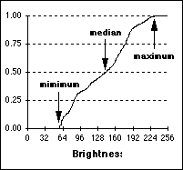
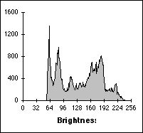
(a) (b)
Figure
6:
(a) Brightness distribution function of Figure 4a with minimum, median,
and maximum indicated. See text for explanation. (b) Brightness
histogram of Figure 4a.
Both
the distribution function and the histogram as measured from a region
are a statistical description of that region. It must be emphasized that
both P[a] and p[a] should be viewed as estimates
of true distributions when they are computed from a specific region.
That is, we view an image and a specific region as one realization of
the various random processes involved in the formation of that image and
that region. In the same context, the statistics defined below must be
viewed as estimates of the underlying parameters.
Average
The average brightness of a
region is defined as the sample mean of the pixel
brightnesses within that region. The average, ma, of
the brightnesses over the
![]() pixels
within a region (
pixels
within a region (
![]() )
is given by:
)
is given by:
![]()
Alternatively,
we can use a formulation based upon the (unnormalized) brightness
histogram, h(a) =
![]() *p(a), with discrete brightness
values a. This gives:
*p(a), with discrete brightness
values a. This gives:
![]()
The
average brightness, ma, is an estimate of the mean
brightness, ua, of the underlying brightness probability
distribution.
Standard deviation
The unbiased estimate
of the standard deviation, sa, of the brightnesses
within a region (
![]() )
with
)
with
![]() pixels
is called the sample standard deviation and is
given by:
pixels
is called the sample standard deviation and is
given by:
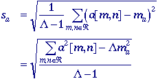
Using
the histogram formulation gives:

The
standard deviation, sa, is an estimate of
![]() a
of the underlying brightness probability distribution.
a
of the underlying brightness probability distribution.
Coefficient-of-variation
The dimensionless coefficient-of-variation, CV, is defined as:
![]()
Percentiles
The percentile, p%, of an unquantized brightness distribution is defined as that value of the brightness a such that:
P(a) = p%
or equivalently
![]()
Three
special cases are frequently used in digital image processing.
*
0% the minimum value in the region
*
50% the median value in the region
*
100% the maximum value in the region
All
three of these values can be determined from Figure 6a.
Mode
The mode of the distribution is the most frequent brightness value. There is no guarantee that a mode exists or that it is unique.
SignaltoNoise ratio
The signal-to-noise ratio, SNR, can have several definitions. The noise is characterized by its standard deviation, sn. The characterization of the signal can differ. If the signal is known to lie between two boundaries, amin <= a <= amax, then the SNR is defined as:
Bounded
signal -

If
the signal is not bounded but has a statistical distribution then two
other definitions are known:
Stochastic
signal - S & N inter-dependent

S
& N independent

where
ma and sa are defined above.
The
various statistics are given in Table 5 for the image and the region
shown in Figure 7.

 Figure
7 Table 5 Region is the interior of the circle. Statistics from Figure 7
A
SNR calculation for the entire image based on eq. is not
directly available. The variations in the image brightnesses that lead
to the large value of s (=49.5) are not, in general, due to noise
but to the variation in local information. With the help of the region
there is a way to estimate the SNR. We can use the s
![]() (=4.0) and the dynamic range, amax - amin,
for the image (=241-56) to calculate a global SNR (=33.3 dB). The
underlying assumptions are that 1) the signal is approximately constant
in that region and the variation in the region is therefore due to
noise, and, 2) that the noise is the same over the entire image with a
standard deviation given by sn = s
(=4.0) and the dynamic range, amax - amin,
for the image (=241-56) to calculate a global SNR (=33.3 dB). The
underlying assumptions are that 1) the signal is approximately constant
in that region and the variation in the region is therefore due to
noise, and, 2) that the noise is the same over the entire image with a
standard deviation given by sn = s
![]() .
.
 Contour Representations
![]()
When
dealing with a region or object, several compact representations are
available that can facilitate manipulation of and measurements on the
object. In each case we assume that we begin with an image
representation of the object as shown in Figure 8a,b. Several techniques
exist to represent the region or object by describing its contour.
Chain code
This representation is based upon the work of Freeman . We follow the contour in a clockwise manner and keep track of the directions as we go from one contour pixel to the next. For the standard implementation of the chain code we consider a contour pixel to be an object pixel that has a background (non-object) pixel as one or more of its 4-connected neighbors. See Figures 3a and 8c.
The
codes associated with eight possible directions are the chain codes and,
with x as the current contour pixel position, the codes are
generally defined as:


Figure
8:
Region (shaded) as it is transformed from (a) continuous to (b) discrete
form and then considered as a (c) contour or (d) run lengths illustrated
in alternating colors.
Chain code properties
* Even codes {0,2,4,6} correspond to horizontal and vertical directions; odd codes {1,3,5,7} correspond to the diagonal directions.
*
Each code can be considered as the angular direction, in multiples of 45deg.,
that we must move to go from one contour pixel to the next.
*
The absolute coordinates [m,n] of the first contour pixel
(e.g. top, leftmost) together with the chain code of the contour
represent a complete description of the discrete region contour.
*
When there is a change between two consecutive chain codes, then the
contour has changed direction. This point is defined as a corner.
Crack code
An alternative to the chain code for contour encoding is to use neither the contour pixels associated with the object nor the contour pixels associated with background but rather the line, the "crack", in between. This is illustrated with an enlargement of a portion of Figure 8 in Figure 9.
The
"crack" code can be viewed as a chain code with four possible
directions instead of eight.

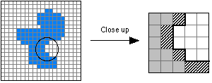 (a)
(b)
Figure
9:
(a) Object including part to be studied. (b) Contour pixels as used in
the chain code are diagonally shaded. The "crack" is shown
with the thick black line.
The
chain code for the enlarged section of Figure 9b, from top to bottom, is
{5,6,7,7,0}. The crack code is {3,2,3,3,0,3,0,0}.
Run codes
A third representation is based on coding the consecutive pixels along a row--a run--that belong to an object by giving the starting position of the run and the ending position of the run. Such runs are illustrated in Figure 8d. There are a number of alternatives for the precise definition of the positions. Which alternative should be used depends upon the application and thus will not be discussed here.


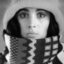

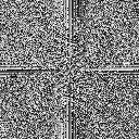
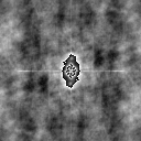
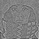 Figure 5a Figure
5b


