Algorithms

Histogram-based Operations

An important class of point operations is based upon the manipulation of an image histogram or a region histogram. The most important examples are described below.

Contrast stretching

Frequently, an image is scanned in such a way that the resulting brightness values do not make full use of the available dynamic range. This can be easily observed in the histogram of the brightness values shown in Figure 6. By stretching the histogram over the available dynamic range we attempt to correct this situation. If the image is intended to go from brightness 0 to brightness 2^B-1 (see Section 2.1), then one generally maps the 0% value (or minimum as defined in Section 3.5.2) to the value 0 and the 100% value (or maximum) to the value 2^B-1. The appropriate transformation is given by:

This formula, however, can be somewhat sensitive to outliers and a less sensitive and more general version is given by:

In this second version one might choose the 1% and 99% values for p_low% and p_high%, respectively, instead of the 0% and 100% values represented by eq. . It is also possible to apply the contrast-stretching operation on a regional basis using the histogram from a region to determine the appropriate limits for the algorithm. Note that in eqs. and it is possible to suppress the term 2^B-1 and simply normalize the brightness range to 0 <= b[m,n] <= 1. This means representing the final pixel brightnesses as reals instead of integers but modern computer speeds and RAM capacities make this quite feasible.

Equalization

When one wishes to compare two or more images on a specific basis, such as texture, it is common to first normalize their histograms to a "standard" histogram. This can be especially useful when the images have been acquired under different circumstances. The most common histogram normalization technique is histogram equalization where one attempts to change the histogram through the use of a function b = f (a) into a histogram that is constant for all brightness values. This would correspond to a brightness distribution where all values are equally probable. Unfortunately, for an arbitrary image, one can only approximate this result.

For a "suitable" function f (a) the relation between the input probability density function, the output probability density function, and the function f (a) is given by:

From eq. we see that "suitable" means that f (a) is differentiable and that df/da >= 0. For histogram equalization we desire that p_b(b) = constant and this means that:

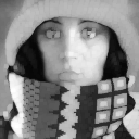
where P(a) is the probability distribution function defined in Section 3.5.1 and illustrated in Figure 6a. In other words, the quantized probability distribution function normalized from 0 to 2^B-1 is the look-up table required for histogram equalization. Figures 21a-c illustrate the effect of contrast stretching and histogram equalization on a standard image. The histogram equalization procedure can also be applied on a regional basis.

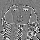
Figure 21a Figure 21b Figure 21c Original Contrast Stretched istogram Equalized

Other histogram-based operations

The histogram derived from a local region can also be used to drive local filters that are to be applied to that region. Examples include minimum filtering, median filtering, and maximum filtering . The concepts minimum, median, and maximum were introduced in Figure 6. The filters based on these concepts will be presented formally in Sections 9.4.2 and 9.6.10.

Mathematics-based Operations

We distinguish in this section between binary arithmetic and ordinary arithmetic. In the binary case there are two brightness values "0" and "1". In the ordinary case we begin with 2^B brightness values or levels but the processing of the image can easily generate many more levels. For this reason many software systems provide 16 or 32 bit representations for pixel brightnesses in order to avoid problems with arithmetic overflow.

Binary operations

Operations based on binary (Boolean) arithmetic form the basis for a powerful set of tools that will be described here and extended in Section 9.6, mathematical morphology. The operations described below are point operations and thus admit a variety of efficient implementations including simple look-up tables. The standard notation for the basic set of binary operations is:

The implication is that each operation is applied on a pixel-by-pixel basis. For example, . The definition of each operation is:

These operations are illustrated in Figure 22 where the binary value "1" is shown in black and the value "0" in white.

a) Image a b) Image b

c) NOT(b) = d) OR(a,b) = a + b e) AND(a,b) = a * b

f) XOR(a,b) = a b g) SUB(a,b) = a \ b

Figure 22: Examples of the various binary point operations.

The SUB(*) operation can be particularly useful when the image a represents a region-of-interest that we want to analyze systematically and the image b represents objects that, having been analyzed, can now be discarded, that is subtracted, from the region.

Arithmetic-based operations

The gray-value point operations that form the basis for image processing are based on ordinary mathematics and include:

 Convolution-based Operations

Convolution, the mathematical, local operation defined in Section 3.1 is central to modern image processing. The basic idea is that a window of some finite size and shape--the support--is scanned across the image. The output pixel value is the weighted sum of the input pixels within the window where the weights are the values of the filter assigned to every pixel of the window itself. The window with its weights is called the convolution kernel. This leads directly to the following variation on eq. . If the filter h[j,k] is zero outside the (rectangular) window {j=0,1,...,J-1; k=0,1,...,K-1}, then, using eq. , the convolution can be written as the following finite sum:

This equation can be viewed as more than just a pragmatic mechanism for smoothing or sharpening an image. Further, while eq. illustrates the local character of this operation, eqs. and suggest that the operation can be implemented through the use of the Fourier domain which requires a global operation, the Fourier transform. Both of these aspects will be discussed below.

Background

In a variety of image-forming systems an appropriate model for the transformation of the physical signal a(x,y) into an electronic signal c(x,y) is the convolution of the input signal with the impulse response of the sensor system. This system might consist of both an optical as well as an electrical sub-system. If each of these systems can be treated as a linear, shift-invariant (LSI) system then the convolution model is appropriate. The definitions of these two, possible, system properties are given below:

Linearity -

Shift-Invariance -

where w₁ and w₂ are arbitrary complex constants and x_o and y_o are coordinates corresponding to arbitrary spatial translations.

Two remarks are appropriate at this point. First, linearity implies (by choosing w₁ = w₂ = 0) that "zero in" gives "zero out". The offset described in eq. means that such camera signals are not the output of a linear system and thus (strictly speaking) the convolution result is not applicable. Fortunately, it is straightforward to correct for this non-linear effect. (See Section 10.1.)

Second, optical lenses with a magnification, M, other than 1x are not shift invariant; a translation of 1 unit in the input image a(x,y) produces a translation of M units in the output image c(x,y). Due to the Fourier property described in eq. this case can still be handled by linear system theory.

If an impulse point of light d(x,y) is imaged through an LSI system then the impulse response of that system is called the point spread function (PSF). The output image then becomes the convolution of the input image with the PSF. The Fourier transform of the PSF is called the optical transfer function (OTF). For optical systems that are circularly-symmetric, aberration-free, and diffraction-limited the PSF is given by the Airy disk shown in Table 4-T.5. The OTF of the Airy disk is also presented in Table 4-T.5.

If the convolution window is not the diffraction-limited PSF of the lens but rather the effect of defocusing a lens then an appropriate model for h(x,y) is a pill box of radius a as described in Table 4-T.3. The effect on a test pattern is illustrated in Figure 23.

a) Test pattern b) Defocused image

Figure 23: Convolution of test pattern with a pill box of radius a=4.5 pixels.

The effect of the defocusing is more than just simple blurring or smoothing. The almost periodic negative lobes in the transfer function in Table 4-T.3 produce a 180deg. phase shift in which black turns to white and vice-versa. The phase shift is clearly visible in Figure 23b.

Convolution in the spatial domain

In describing filters based on convolution we will use the following convention. Given a filter h[j,k] of dimensions J x K, we will consider the coordinate [j=0,k=0] to be in the center of the filter matrix, h. This is illustrated in Figure 24. The "center" is well-defined when J and K are odd; for the case where they are even, we will use the approximations (J/2, K/2) for the "center" of the matrix.

Figure 24: Coordinate system for describing h[j,k]

When we examine the convolution sum (eq. ) closely, several issues become evident.

* Evaluation of formula for m=n=0 while rewriting the limits of the convolution sum based on the "centering" of h[j,k] shows that values of a[j,k] can be required that are outside the image boundaries:

The question arises - what values should we assign to the image a[m,n] for m<0, m>=M, n<0, and n>=N? There is no "answer" to this question. There are only alternatives among which we are free to choose assuming we understand the possible consequences of our choice. The standard alternatives are a) extend the images with a constant (possibly zero) brightness value, b) extend the image periodically, c) extend the image by mirroring it at its boundaries, or d) extend the values at the boundaries indefinitely. These alternatives are illustrated in Figure 25.

(a) (b) (c) (d)

Figure 25: Examples of various alternatives to extend an image outside its formal boundaries. See text for explanation.

* When the convolution sum is written in the standard form (eq. ) for an image a[m,n] of size M x N:

we see that the convolution kernel h[j,k] is mirrored around j=k=0 to produce
h[-j,-k] before it is translated by [m,n] as indicated in eq. . While some convolution kernels in common use are symmetric in this respect, h[j,k]= h[-j,-k], many are not. (See Section 9.5.) Care must therefore be taken in the implementation of filters with respect to the mirroring requirements.

* The computational complexity for a K x K convolution kernel implemented in the spatial domain on an image of N x N is O(K²) where the complexity is measured per pixel on the basis of the number of multiplies-and-adds (MADDs).

* The value computed by a convolution that begins with integer brightnesses for a[m,n] may produce a rational number or a floating point number in the result c[m,n]. Working exclusively with integer brightness values will, therefore, cause roundoff errors.

* Inspection of eq. reveals another possibility for efficient implementation of convolution. If the convolution kernel h[j,k] is separable, that is, if the kernel can be written as:

then the filtering can be performed as follows:

This means that instead of applying one, two-dimensional filter it is possible to apply two, one-dimensional filters, the first one in the k direction and the second one in the j direction. For an N x N image this, in general, reduces the computational complexity per pixel from O(J* K) to O(J+K).

An alternative way of writing separability is to note that the convolution kernel (Figure 24) is a matrix h and, if separable, h can be written as:

where "^t" denotes the matrix transpose operation. In other words, h can be expressed as the outer product of a column vector [h_col] and a row vector [h_row].

* For certain filters it is possible to find an incremental implementation for a convolution. As the convolution window moves over the image (see eq. ), the leftmost column of image data under the window is shifted out as a new column of image data is shifted in from the right. Efficient algorithms can take advantage of this and, when combined with separable filters as described above, this can lead to algorithms where the computational complexity per pixel is O(constant).

Convolution in the frequency domain

In Section 3.4 we indicated that there was an alternative method to implement the filtering of images through convolution. Based on eq. it appears possible to achieve the same result as in eq. by the following sequence of operations:

i) Compute A( , ) = F{a[m,n]}

ii) Multiply A( , ) by the precomputed ( , ) = F{h[m,n]}

iii) Compute the result c[m,n] = F^-1{A( , )*( , )}

* While it might seem that the "recipe" given above in eq. circumvents the problems associated with direct convolution in the spatial domain--specifically, determining values for the image outside the boundaries of the image--the Fourier domain approach, in fact, simply "assumes" that the image is repeated periodically outside its boundaries as illustrated in Figure 25b. This phenomenon is referred to as circular convolution.

If circular convolution is not acceptable then the other possibilities illustrated in Figure 25 can be realized by embedding the image a[m,n] and the filter ( , ) in larger matrices with the desired image extension mechanism for a[m,n] being explicitly implemented.

* The computational complexity per pixel of the Fourier approach for an image of N x N and for a convolution kernel of K x K is O(logN) complex MADDs independent of K. ere we assume that N > K and that N is a highly composite number such as a power of two. (See also 2.1.) This latter assumption permits use of the computationally-efficient Fast Fourier Transform (FFT) algorithm. Surprisingly then, the indirect route described by eq. can be faster than the direct route given in eq. . This requires, in general, that K² >> logN. The range of K and N for which this holds depends on the specifics of the implementation. For the machine on which this manuscript is being written and the specific image processing package that is being used, for an image of N = 256 the Fourier approach is faster than the convolution approach when K >= 15. (It should be noted that in this comparison the direct convolution involves only integer arithmetic while the Fourier domain approach requires complex floating point arithmetic.)

Smoothing Operations

These algorithms are applied in order to reduce noise and/or to prepare images for further processing such as segmentation. We distinguish between linear and non- linear algorithms where the former are amenable to analysis in the Fourier domain and the latter are not. We also distinguish between implementations based on a rectangular support for the filter and implementations based on a circular support for the filter.

Linear Filters

Several filtering algorithms will be presented together with the most useful supports.

* Uniform filter - The output image is based on a local averaging of the input filter where all of the values within the filter support have the same weight. In the continuous spatial domain (x,y) the PSF and transfer function are given in Table 4-T.1 for the rectangular case and in Table 4-T.3 for the circular (pill box) case. For the discrete spatial domain [m,n] the filter values are the samples of the continuous domain case. Examples for the rectangular case (J=K=5) and the circular case (R=2.5) are shown in Figure 26.

(a) Rectangular filter (J=K=5) (b) Circular filter (R=2.5)

Figure 26: Uniform filters for image smoothing

Note that in both cases the filter is normalized so that h[j,k] = 1. This is done so that if the input a[m,n] is a constant then the output image c[m,n] is the same constant. The justification can be found in the Fourier transform property described in eq. . As can be seen from Table 4, both of these filters have transfer functions that have negative lobes and can, therefore, lead to phase reversal as seen in Figure 23. The square implementation of the filter is separable and incremental; the circular implementation is incremental .

* Triangular filter - The output image is based on a local averaging of the input filter where the values within the filter support have differing weights. In general, the filter can be seen as the convolution of two (identical) uniform filters either rectangular or circular and this has direct consequences for the computational complexity . (See Table 13.) In the continuous spatial domain the PSF and transfer function are given in Table 4-T.2 for the rectangular support case and in Table 4-T.4 for the circular (pill box) support case. As seen in Table 4 the transfer functions of these filters do not have negative lobes and thus do not exhibit phase reversal.

Examples for the rectangular support case (J=K=5) and the circular support case (R=2.5) are shown in Figure 27. The filter is again normalized so that h[j,k]=1.

(a) Pyramidal filter (J=K=5) (b) Cone filter (R=2.5)

Figure 27: Triangular filters for image smoothing

* Gaussian filter - The use of the Gaussian kernel for smoothing has become extremely popular. This has to do with certain properties of the Gaussian (e.g. the central limit theorem, minimum space-bandwidth product) as well as several application areas such as edge finding and scale space analysis. The PSF and transfer function for the continuous space Gaussian are given in Table 4-T6. The Gaussian filter is separable:

There are four distinct ways to implement the Gaussian:

- Convolution using a finite number of samples (N_o) of the Gaussian as the convolution kernel. It is common to choose N_o = 3 or 5 .

- Repetitive convolution using a uniform filter as the convolution kernel.

The actual implementation (in each dimension) is usually of the form:

This implementation makes use of the approximation afforded by the central limit theorem. For a desired with eq. , we use N_o = although this severely restricts our choice of 's to integer values.

- Multiplication in the frequency domain. As the Fourier transform of a Gaussian is a Gaussian (see Table -T.6), this means that it is straightforward to prepare a filter ( , ) = G_2D( , ) for use with eq. . To avoid truncation effects in the frequency domain due to the infinite extent of the Gaussian it is important to choose a that is sufficiently large. Choosing > k/ where k = 3 or 4 will usually be sufficient.

- Use of a recursive filter implementation. A recursive filter has an infinite impulse response and thus an infinite support. The separable Gaussian filter can also be implemented by applying the following recipe in each dimension when >= 0.5.

i) Choose the based on the desired goal of the filtering; ii) Determine the parameter q based on eq. ; iii) Use eq. to determine the filter coefficients {b₀,b₁,b₂,b₃,B}; iv) Apply the forward difference equation, eq. ; v) Apply the backward difference equation, eq. ;

The relation between the desired and q is given by:

The filter coefficients {b₀,b₁,b₂,b₃,B} are defined by:

The one-dimensional forward difference equation takes an input row (or column) a[n] and produces an intermediate output result w[n] given by:

The one-dimensional backward difference equation takes the intermediate result w[n] and produces the output c[n] given by:

The forward equation is applied from n = 0 up to n = N - 1 while the backward equation is applied from n = N - 1 down to n = 0.

The relative performance of these various implementation of the Gaussian filter can be described as follows. Using the root-square error between a true, infinite-extent Gaussian, g[n| ], and an approximated Gaussian, h[n], as a measure of accuracy, the various algorithms described above give the results shown in Figure. 28a. The relative speed of the various algorithms in shown in Figure 28b.

The root-square error measure is extremely conservative and thus all filters, with the exception of "Uniform 3x" for large , are sufficiently accurate. The recursive implementation is the fastest independent of ; the other implementations can be significantly slower. The FFT implementation, for example, is 3.1 times slower for N=256 . Further, the FFT requires that N be a highly composite number.

a) Accuracy comparison b) Speed comparison

Figure 28: Comparison of various Gaussian algorithms with N=256. The legend is spread across both graphs

* Other - The Fourier domain approach offers the opportunity to implement a variety of smoothing algorithms. The smoothing filters will then be lowpass filters. In general it is desirable to use a lowpass filter that has zero phase so as not to produce phase distortion when filtering the image. The importance of phase was illustrated in Figures 5 and 23. When the frequency domain characteristics can be represented in an analytic form, then this can lead to relatively straightforward implementations of ( , ). Possible candidates include the lowpass filters "Airy" and "Exponential Decay" found in Table 4-T.5 and Table 4-T.8, respectively.

Non-Linear Filters

A variety of smoothing filters have been developed that are not linear. While they cannot, in general, be submitted to Fourier analysis, their properties and domains of application have been studied extensively.

* Median filter - The median statistic was described in Section 3.5.2. A median filter is based upon moving a window over an image (as in a convolution) and computing the output pixel as the median value of the brightnesses within the input window. If the window is J x K in size we can order the J*K pixels in brightness value from smallest to largest. If J*K is odd then the median will be the (J*K+1)/2 entry in the list of ordered brightnesses. Note that the value selected will be exactly equal to one of the existing brightnesses so that no roundoff error will be involved if we want to work exclusively with integer brightness values. The algorithm as it is described above has a generic complexity per pixel of O(J*K*log(J*K)). Fortunately, a fast algorithm (due to uang et al. ) exists that reduces the complexity to O(K) assuming J >= K.

A useful variation on the theme of the median filter is the percentile filter. ere the center pixel in the window is replaced not by the 50% (median) brightness value but rather by the p% brightness value where p% ranges from 0% (the minimum filter) to 100% (the maximum filter). Values other then (p=50)% do not, in general, correspond to smoothing filters.

* Kuwahara filter - Edges play an important role in our perception of images (see Figure 15) as well as in the analysis of images. As such it is important to be able to smooth images without disturbing the sharpness and, if possible, the position of edges. A filter that accomplishes this goal is termed an edge-preserving filter and one particular example is the Kuwahara filter . Although this filter can be implemented for a variety of different window shapes, the algorithm will be described for a square window of size J = K = 4L + 1 where L is an integer. The window is partitioned into four regions as shown in Figure 29.

Figure 29: Four, square regions defined for the Kuwahara filter. In this example L=1 and thus J=K=5. Each region is [(J+1)/2] x [(K+1)/2].

In each of the four regions (i=1,2,3,4), the mean brightness, m_i in eq. , and the variance_i, s_i² in eq. , are measured. The output value of the center pixel in the window is the mean value of that region that has the smallest variance.

Summary of Smoothing Algorithms

The following table summarizes the various properties of the smoothing algorithms presented above. The filter size is assumed to be bounded by a rectangle of J x K where, without loss of generality, J >= K. The image size is N x N.

Table 13: Characteristics of smoothing filters. ªSee text for additional explanation.

Examples of the effect of various smoothing algorithms are shown in Figure 30.

a) Original b) Uniform 5 x 5 c) Gaussian ( = 2.5)

d) Median 5 x 5 e) Kuwahara 5 x 5

Figure 30: Illustration of various linear and non-linear smoothing filters

Derivative-based Operations

Just as smoothing is a fundamental operation in image processing so is the ability to take one or more spatial derivatives of the image. The fundamental problem is that, according to the mathematical definition of a derivative, this cannot be done. A digitized image is not a continuous function a(x,y) of the spatial variables but rather a discrete function a[m,n] of the integer spatial coordinates. As a result the algorithms we will present can only be seen as approximations to the true spatial derivatives of the original spatially-continuous image.

Further, as we can see from the Fourier property in eq. , taking a derivative multiplies the signal spectrum by either u or v. This means that high frequency noise will be emphasized in the resulting image. The general solution to this problem is to combine the derivative operation with one that suppresses high frequency noise, in short, smoothing in combination with the desired derivative operation.

First Derivatives

As an image is a function of two (or more) variables it is necessary to define the direction in which the derivative is taken. For the two-dimensional case we have the horizontal direction, the vertical direction, or an arbitrary direction which can be considered as a combination of the two. If we use h_x to denote a horizontal derivative filter (matrix), h_y to denote a vertical derivative filter (matrix), and h to denote the arbitrary angle derivative filter (matrix), then:

* Gradient filters - It is also possible to generate a vector derivative description as the gradient, a[m,n], of an image:

where are unit vectors in the horizontal and vertical direction, respectively. This leads to two descriptions:

Gradient magnitude -

and

Gradient direction -

The gradient magnitude is sometimes approximated by:

Approx. Gradient magnitude -

The final results of these calculations depend strongly on the choices of h_x and h_y. A number of possible choices for (h_x, h_y) will now be described.

* Basic derivative filters - These filters are specified by:

where "^t" denotes matrix transpose. These two filters differ significantly in their Fourier magnitude and Fourier phase characteristics. For the frequency range 0 <= <= , these are given by:

The second form (ii) gives suppression of high frequency terms ( ~ ) while the first form (i) does not. The first form leads to a phase shift; the second form does not.

* Prewitt gradient filters - These filters are specified by:

Both h_x and h_y are separable. Beyond the computational implications are the implications for the analysis of the filter. Each filter takes the derivative in one direction using eq. ii and smoothes in the orthogonal direction using a one-dimensional version of a uniform filter as described in Section 9.4.1.

* Sobel gradient filters - These filters are specified by:

Again, h_x and h_y are separable. Each filter takes the derivative in one direction using eq. ii and smoothes in the orthogonal direction using a one-dimensional version of a triangular filter as described in Section 9.4.1.

* Alternative gradient filters - The variety of techniques available from one-dimensional signal processing for the design of digital filters offers us powerful tools for designing one-dimensional versions of h_x and h_y. Using the Parks-McClellan filter design algorithm, for example, we can choose the frequency bands where we want the derivative to be taken and the frequency bands where we want the noise to be suppressed. The algorithm will then produce a real, odd filter with a minimum length that meets the specifications.

As an example, if we want a filter that has derivative characteristics in a passband (with weight 1.0) in the frequency range 0.0 <= <= 0.3 and a stopband (with weight 3.0) in the range 0.32 <= <= , then the algorithm produces the following optimized seven sample filter:

The gradient can then be calculated as in eq. .

* Gaussian gradient filters - In modern digital image processing one of the most common techniques is to use a Gaussian filter (see Section 9.4.1) to accomplish the required smoothing and one of the derivatives listed in eq. . Thus, we might first apply the recursive Gaussian in eq. followed by eq. ii to achieve the desired, smoothed derivative filters h_x and h_y. Further, for computational efficiency, we can combine these two steps as:

where the various coefficients are defined in eq. . The first (forward) equation is applied from n = 0 up to n = N - 1 while the second (backward) equation is applied from n = N - 1 down to n = 0.

* Summary - Examples of the effect of various derivative algorithms on a noisy version of Figure 30a (SNR = 29 dB) are shown in Figure 31a-c. The effect of various magnitude gradient algorithms on Figure 30a are shown in Figure 32a-c. After processing, all images are contrast stretched as in eq. for display purposes.

(a) (b) (c) Simple Derivative - eq. ii Sobel - eq. Gaussian ( =1.5) & eq. ii

Figure 31: Application of various algorithms for h_x - the horizontal derivative.

(a) (b) (c) Simple Derivative - eq. ii Sobel - eq. Gaussian ( =1.5) & eq. ii

Figure 32: Various algorithms for the magnitude gradient, | a|.

The magnitude gradient takes on large values where there are strong edges in the image. Appropriate choice of in the Gaussian-based derivative (Figure 31c) or gradient (Figure 32c) permits computation of virtually any of the other forms - simple, Prewitt, Sobel, etc. In that sense, the Gaussian derivative represents a superset of derivative filters.

Second Derivatives

It is, of course, possible to compute higher-order derivatives of functions of two variables. In image processing, as we shall see in Sections 10.2.1 and 10.3.2, the second derivatives or Laplacian play an important role. The Laplacian is defined as:

where h_2x and h_2y are second derivative filters. In the frequency domain we have for the Laplacian filter (from eq. ):

The transfer function of a Laplacian corresponds to a parabola (u,v) = -(u² + v²).

* Basic second derivative filter - This filter is specified by:

and the frequency spectrum of this filter, in each direction, is given by:

over the frequency range - <= <= . The two, one-dimensional filters can be used in the manner suggested by eq. or combined into one, two-dimensional filter as:

and used as in eq. .

* Frequency domain Laplacian - This filter is the implementation of the general recipe given in eq. and for the Laplacian filter takes the form:

* Gaussian second derivative filter - This is the straightforward extension of the Gaussian first derivative filter described above and can be applied independently in each dimension. We first apply Gaussian smoothing with a chosen on the basis of the problem specification. We then apply the desired second derivative filter eq. or eq. . Again there is the choice among the various Gaussian smoothing algorithms.

For efficiency, we can use the recursive implementation and combine the two steps--smoothing and derivative operation--as follows:

where the various coefficients are defined in eq. . Again, the first (forward) equation is applied from n = 0 up to n = N - 1 while the second (backward) equation is applied from n = N - 1 down to n = 0.

* Alternative Laplacian filters - Again one-dimensional digital filter design techniques offer us powerful methods to create filters that are optimized for a specific problem. Using the Parks-McClellan design algorithm, we can choose the frequency bands where we want the second derivative to be taken and the frequency bands where we want the noise to be suppressed. The algorithm will then produce a real, even filter with a minimum length that meets the specifications.

As an example, if we want a filter that has second derivative characteristics in a passband (with weight 1.0) in the frequency range 0.0 <= <= 0.3 and a stopband (with weight 3.0) in the range 0.32 <= <= , then the algorithm produces the following optimized seven sample filter:

The Laplacian can then be calculated as in eq. .

* SDGD filter - A filter that is especially useful in edge finding and object measurement is the Second-Derivative-in-the-Gradient-Direction (SDGD) filter. This filter uses five partial derivatives:

Note that A_xy = A_yx which accounts for the five derivatives.

This SDGD combines the different partial derivatives as follows:

As one might expect, the large number of derivatives involved in this filter implies that noise suppression is important and that Gaussian derivative filters--both first and second order--are highly recommended if not required . It is also necessary that the first and second derivative filters have essentially the same passbands and stopbands. This means that if the first derivative filter h_1x is given by [1 0 -1] (eq. ii) then the second derivative filter should be given by h_1x h_1x = h_2x = [1 0 -2 0 1].

* Summary - The effects of the various second derivative filters are illustrated in Figure 33a-e. All images were contrast stretched for display purposes using eq. and the parameters 1% and 99%.

(a) (b) (c) Laplacian - eq. Fourier parabola - eq. Gaussian ( =1.0) & eq.

(d) (e) "Designer" - eq. SDGD ( =1.0) - eq.

Figure 33: Various algorithms for the Laplacian and Laplacian-related filters.

Other Filters

An infinite number of filters, both linear and non-linear, are possible for image processing. It is therefore impossible to describe more than the basic types in this section. The description of others can be found be in the reference literature (see Section 11) as well as in the applications literature. It is important to use a small consistent set of test images that are relevant to the application area to understand the effect of a given filter or class of filters. The effect of filters on images can be frequently understood by the use of images that have pronounced regions of varying sizes to visualize the effect on edges or by the use of test patterns such as sinusoidal sweeps to visualize the effects in the frequency domain. The former have been used above (Figures 21, 23, and 30-33) and the latter are demonstrated below in Figure 34.

(a) Lowpass filter (b) Bandpass filter (c) ighpass filter

Figure 34: Various convolution algorithms applied to sinusoidal test image.

Morphology-based Operations

In Section 1 we defined an image as an (amplitude) function of two, real (coordinate) variables a(x,y) or two, discrete variables a[m,n]. An alternative definition of an image can be based on the notion that an image consists of a set (or collection) of either continuous or discrete coordinates. In a sense the set corresponds to the points or pixels that belong to the objects in the image. This is illustrated in Figure 35 which contains two objects or sets A and B. Note that the coordinate system is required. For the moment we will consider the pixel values to be binary as discussed in Section 2.1 and 9.2.1. Further we shall restrict our discussion to discrete space (Z²). More general discussions can be found in .

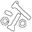
Figure 35: A binary image containing two object sets A and B.

The object A consists of those pixels a that share some common property:

Object -

As an example, object B in Figure 35 consists of {[0,0], [1,0], [0,1]}.

The background of A is given by A^c (the complement of A) which is defined as those elements that are not in A:

Background -

In Figure 3 we introduced the concept of neighborhood connectivity. We now observe that if an object A is defined on the basis of C-connectivity (C=4, 6, or 8) then the background A^c has a connectivity given by 12 - C. The necessity for this is illustrated for the Cartesian grid in Figure 36.

Figure 36: A binary image requiring careful definition of object and background connectivity.

Fundamental definitions

The fundamental operations associated with an object are the standard set operations union, intersection, and complement { , , ^c} plus translation:

* Translation - Given a vector x and a set A, the translation, A + x, is defined as:

Note that, since we are dealing with a digital image composed of pixels at integer coordinate positions (Z²), this implies restrictions on the allowable translation vectors x.

The basic Minkowski set operations--addition and subtraction--can now be defined. First we note that the individual elements that comprise B are not only pixels but also vectors as they have a clear coordinate position with respect to [0,0]. Given two sets A and B:

Minkowski addition -

Minkowski subtraction -

Dilation and Erosion

From these two Minkowski operations we define the fundamental mathematical morphology operations dilation and erosion:

Dilation -

Erosion -

where . These two operations are illustrated in Figure 37 for the objects defined in Figure 35.

(a) Dilation D(A,B) (b) Erosion E(A,B)

Figure 37: A binary image containing two object sets A and B. The three pixels in B are "color-coded" as is their effect in the result.

While either set A or B can be thought of as an "image", A is usually considered as the image and B is called a structuring element. The structuring element is to mathematical morphology what the convolution kernel is to linear filter theory.

Dilation, in general, causes objects to dilate or grow in size; erosion causes objects to shrink. The amount and the way that they grow or shrink depend upon the choice of the structuring element. Dilating or eroding without specifying the structural element makes no more sense than trying to lowpass filter an image without specifying the filter. The two most common structuring elements (given a Cartesian grid) are the 4-connected and 8-connected sets, N₄ and N₈. They are illustrated in Figure 38.

(a) N₄ (b) N₈

Figure 38: The standard structuring elements N₄ and N₈.

Dilation and erosion have the following properties:

Commutative -

Non-Commutative -

Associative -

Translation Invariance -

Duality -

With A as an object and A^c as the background, eq. says that the dilation of an object is equivalent to the erosion of the background. Likewise, the erosion of the object is equivalent to the dilation of the background.

Except for special cases:

Non-Inverses -

Erosion has the following translation property:

Translation Invariance -

Dilation and erosion have the following important properties. For any arbitrary structuring element B and two image objects A₁ and A₂ such that A₁ A₂ (A₁ is a proper subset of A₂):

Increasing in A -

For two structuring elements B₁ and B₂ such that B₁ B₂:

Decreasing in B -

The decomposition theorems below make it possible to find efficient implementations for morphological filters.

Dilation -

Erosion -

Erosion -

Multiple Dilations -

An important decomposition theorem is due to Vincent . First, we require some definitions. A convex set (in R²) is one for which the straight line joining any two points in the set consists of points that are also in the set. Care must obviously be taken when applying this definition to discrete pixels as the concept of a "straight line" must be interpreted appropriately in Z². A set is bounded if each of its elements has a finite magnitude, in this case distance to the origin of the coordinate system. A set is symmetric if B = -B. The sets N₄ and N₈ in Figure 38 are examples of convex, bounded, symmetric sets.

Vincent's theorem, when applied to an image consisting of discrete pixels, states that for a bounded, symmetric structuring element B that contains no holes and contains its own center, :

where A is the contour of the object. That is, A is the set of pixels that have a background pixel as a neighbor. The implication of this theorem is that it is not necessary to process all the pixels in an object in order to compute a dilation or (using eq. ) an erosion. We only have to process the boundary pixels. This also holds for all operations that can be derived from dilations and erosions. The processing of boundary pixels instead of object pixels means that, except for pathological images, computational complexity can be reduced from O(N²) to O(N) for an N x N image. A number of "fast" algorithms can be found in the literature that are based on this result . The simplest dilation and erosion algorithms are frequently described as follows.

* Dilation - Take each binary object pixel (with value "1") and set all background pixels (with value "0") that are C-connected to that object pixel to the value "1".

* Erosion - Take each binary object pixel (with value "1") that is C-connected to a background pixel and set the object pixel value to "0".

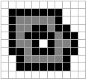
Comparison of these two procedures to eq. where B = N_C=4 or N_C=8 shows that they are equivalent to the formal definitions for dilation and erosion. The procedure is illustrated for dilation in Figure 39.

(a) B = N₄ (b) B= N₈

Figure 39: Illustration of dilation. Original object pixels are in gray; pixels added through dilation are in black.

Boolean Convolution

An arbitrary binary image object (or structuring element) A can be represented as:

where and * are the Boolean operations OR and AND as defined in eqs. (81) and (82), a[j,k] is a characteristic function that takes on the Boolean values "1" and "0" as follows:

and d[m,n] is a Boolean version of the Dirac delta function that takes on the Boolean values "1" and "0" as follows:

Dilation for binary images can therefore be written as:

which, because Boolean OR and AND are commutative, can also be written as

Using De Morgan's theorem:

on eq. together with eq. , erosion can be written as:

Thus, dilation and erosion on binary images can be viewed as a form of convolution over a Boolean algebra.

In Section 9.3.2 we saw that, when convolution is employed, an appropriate choice of the boundary conditions for an image is essential. Dilation and erosion--being a Boolean convolution--are no exception. The two most common choices are that either everything outside the binary image is "0" or everything outside the binary image is "1".

Opening and Closing

We can combine dilation and erosion to build two important higher order operations:

Opening -

Closing -

The opening and closing have the following properties:

Duality -

Translation -

For the opening with structuring element B and images A, A₁, and A₂, where A₁ is a subimage of A₂ (A₁ A₂):

Antiextensivity -

Increasing monotonicity -

Idempotence -

For the closing with structuring element B and images A, A₁, and A₂, where A₁ is a subimage of A₂ (A₁ A₂):

Extensivity -

Increasing monotonicity -

Idempotence -

The two properties given by eqs. and are so important to mathematical morphology that they can be considered as the reason for defining erosion with -B instead of B in eq. .

itandMiss operation

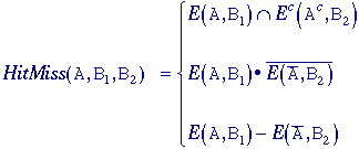
The hit-or-miss operator was defined by Serra but we shall refer to it as the hit-and-miss operator and define it as follows. Given an image A and two structuring elements B₁ and B₂, the set definition and Boolean definition are:

Hit-and-Miss -

where B₁ and B₂ are bounded, disjoint structuring elements. (Note the use of the notation from eq. (81).) Two sets are disjoint if B₁ B₂ = , the empty set. In an important sense the hit-and-miss operator is the morphological equivalent of template matching, a well-known technique for matching patterns based upon cross-correlation. ere, we have a template B₁ for the object and a template B₂ for the background.

Summary of the basic operations

The results of the application of these basic operations on a test image are illustrated below. In Figure 40 the various structuring elements used in the processing are defined. The value "-" indicates a "don't care". All three structuring elements are symmetric.

(a) (b) (c)

Figure 40: Structuring elements B, B₁, and B₂ that are 3 x 3 and symmetric.

The results of processing are shown in Figure 41 where the binary value "1" is shown in black and the value "0" in white.

a) Image A b) Dilation with 2B c) Erosion with 2B

d) Opening with 2B e) Closing with 2B f) it-and-Miss with B₁ and B₂

Figure 41: Examples of various mathematical morphology operations.

The opening operation can separate objects that are connected in a binary image. The closing operation can fill in small holes. Both operations generate a certain amount of smoothing on an object contour given a "smooth" structuring element. The opening smoothes from the inside of the object contour and the closing smoothes from the outside of the object contour. The hit-and-miss example has found the 4-connected contour pixels. An alternative method to find the contour is simply to use the relation:

4-connected contour -

or

8-connected contour -

Skeleton

The informal definition of a skeleton is a line representation of an object that is:

i) one-pixel thick,

ii) through the "middle" of the object, and,

iii) preserves the topology of the object.

These are not always realizable. Figure 42 shows why this is the case.

(a) (b)

Figure 42: Counterexamples to the three requirements.

In the first example, Figure 42a, it is not possible to generate a line that is one pixel thick and in the center of an object while generating a path that reflects the simplicity of the object. In Figure 42b it is not possible to remove a pixel from the 8-connected object and simultaneously preserve the topology--the notion of connectedness--of the object. Nevertheless, there are a variety of techniques that attempt to achieve this goal and to produce a skeleton.

A basic formulation is based on the work of Lantuéjoul . The skeleton subset S_k(A) is defined as:

Skeleton subsets -

where K is the largest value of k before the set S_k(A) becomes empty. (From eq. , ). The structuring element B is chosen (in Z²) to approximate a circular disc, that is, convex, bounded and symmetric. The skeleton is then the union of the skeleton subsets:

Skeleton -

An elegant side effect of this formulation is that the original object can be reconstructed given knowledge of the skeleton subsets S_k(A), the structuring element B, and K:

Reconstruction -

This formulation for the skeleton, however, does not preserve the topology, a requirement described in eq. .

An alternative point-of-view is to implement a thinning, an erosion that reduces the thickness of an object without permitting it to vanish. A general thinning algorithm is based on the hit-and-miss operation:

Thinning -

Depending on the choice of B₁ and B₂, a large variety of thinning algorithms--and through repeated application skeletonizing algorithms--can be implemented.

A quite practical implementation can be described in another way. If we restrict ourselves to a 3 x 3 neighborhood, similar to the structuring element B = N₈ in Figure 40a, then we can view the thinning operation as a window that repeatedly scans over the (binary) image and sets the center pixel to "0" under certain conditions. The center pixel is not changed to "0" if and only if:

i) an isolated pixel is found (e.g. Figure 43a),

ii) removing a pixel would change the connectivity (e.g. Figure 43b),

iii) removing a pixel would shorten a line (e.g. Figure 43c).

As pixels are (potentially) removed in each iteration, the process is called a conditional erosion. Three test cases of eq. are illustrated in Figure 43. In general all possible rotations and variations have to be checked. As there are only 512 possible combinations for a 3 x 3 window on a binary image, this can be done easily with the use of a lookup table.

(a) Isolated pixel (b) Connectivity pixel (c) End pixel

Figure 43: Test conditions for conditional erosion of the center pixel.

If only condition (i) is used then each object will be reduced to a single pixel. This is useful if we wish to count the number of objects in an image. If only condition (ii) is used then holes in the objects will be found. If conditions (i + ii) are used each object will be reduced to either a single pixel if it does not contain a hole or to closed rings if it does contain holes. If conditions (i + ii + iii) are used then the "complete skeleton" will be generated as an approximation to eq. . Illustrations of these various possibilities are given in Figure 44a,b.

Propagation

It is convenient to be able to reconstruct an image that has "survived" several erosions or to fill an object that is defined, for example, by a boundary. The formal mechanism for this has several names including region-filling, reconstruction, and propagation. The formal definition is given by the following algorithm. We start with a seed image S⁽⁰⁾, a mask image A, and a structuring element B. We then use dilations of S with structuring element B and masked by A in an iterative procedure as follows:

Iteration k -

With each iteration the seed image grows (through dilation) but within the set (object) defined by A; S propagates to fill A. The most common choices for B are N₄ or N₈. Several remarks are central to the use of propagation. First, in a straightforward implementation, as suggested by eq. , the computational costs are extremely high. Each iteration requires O(N²) operations for an N x N image and with the required number of iterations this can lead to a complexity of O(N³). Fortunately, a recursive implementation of the algorithm exists in which one or two passes through the image are usually sufficient, meaning a complexity of O(N²). Second, although we have not paid much attention to the issue of object/background connectivity until now (see Figure 36), it is essential that the connectivity implied by B be matched to the connectivity associated with the boundary definition of A (see eqs. and ). Finally, as mentioned earlier, it is important to make the correct choice ("0" or "1") for the boundary condition of the image. The choice depends upon the application.

Summary of skeleton and propagation

The application of these two operations on a test image is illustrated in Figure 44. In Figure 44a,b the skeleton operation is shown with the endpixel condition (eq. i+ii+iii) and without the end pixel condition (eq. i+ii). The propagation operation is illustrated in Figure 44c. The original image, shown in light gray, was eroded by E(A,6N₈) to produce the seed image shown in black. The original was then used as the mask image to produce the final result. The border value in both images was "0".

Several techniques based upon the use of skeleton and propagation operations in combination with other mathematical morphology operations will be given in Section 10.3.3.

Original = light gray Mask = light gray

Skeleton = black Seed = black

a) Skeleton with end pixels b) Skeleton without end pixels c) Propagation with N₈

Condition eq. i+ii+iii Condition eq. i+ii

Figure 44: Examples of skeleton and propagation.

Gray-value morphological processing

The techniques of morphological filtering can be extended to gray-level images. To simplify matters we will restrict our presentation to structuring elements, B, that comprise a finite number of pixels and are convex and bounded. Now, however, the structuring element has gray values associated with every coordinate position as does the image A.

* Gray-level dilation, D_G(*), is given by:

Dilation -

For a given output coordinate [m,n], the structuring element is summed with a shifted version of the image and the maximum encountered over all shifts within the J x K domain of B is used as the result. Should the shifting require values of the image A that are outside the M x N domain of A, then a decision must be made as to which model for image extension, as described in Section 9.3.2, should be used.

* Gray-level erosion, E_G(*), is given by:

Erosion -

The duality between gray-level erosion and gray-level dilation--the gray-level counterpart of eq. --is somewhat more complex than in the binary case:

Duality -

where " " means that a[j,k] -> -a[-j,-k].

The definitions of higher order operations such as gray-level opening and gray-level closing are:

Opening -

Closing -

The important properties that were discussed earlier such as idempotence, translation invariance, increasing in A, and so forth are also applicable to gray level morphological processing. The details can be found in Giardina and Dougherty .

In many situations the seeming complexity of gray level morphological processing is significantly reduced through the use of symmetric structuring elements where b[j,k] = b[-j,-k]. The most common of these is based on the use of B = constant = 0. For this important case and using again the domain [j,k] B, the definitions above reduce to:

Dilation -

Erosion -

Opening -

Closing -

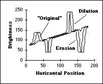
The remarkable conclusion is that the maximum filter and the minimum filter, introduced in Section 9.4.2, are gray-level dilation and gray-level erosion for the specific structuring element given by the shape of the filter window with the gray value "0" inside the window. Examples of these operations on a simple one-dimensional signal are shown in Figure 45.

a) Effect of 15 x 1 dilation and erosion b) Effect of 15 x 1 opening and closing

Figure 45: Morphological filtering of gray-level data.

For a rectangular window, J x K, the two-dimensional maximum or minimum filter is separable into two, one-dimensional windows. Further, a one-dimensional maximum or minimum filter can be written in incremental form. (See Section 9.3.2.) This means that gray-level dilations and erosions have a computational complexity per pixel that is O(constant), that is, independent of J and K. (See also Table 13.)

The operations defined above can be used to produce morphological algorithms for smoothing, gradient determination and a version of the Laplacian. All are constructed from the primitives for gray-level dilation and gray-level erosion and in all cases the maximum and minimum filters are taken over the domain .

Morphological smoothing

This algorithm is based on the observation that a gray-level opening smoothes a gray-value image from above the brightness surface given by the function a[m,n] and the gray-level closing smoothes from below. We use a structuring element B based on eqs. and .

Note that we have suppressed the notation for the structuring element B under the max and min operations to keep the notation simple. Its use, however, is understood.

Morphological gradient

For linear filters the gradient filter yields a vector representation (eq. (103)) with a magnitude (eq. (104)) and direction (eq. (105)). The version presented here generates a morphological estimate of the gradient magnitude:

Morphological Laplacian

The morphologically-based Laplacian filter is defined by:

Summary of morphological filters

The effect of these filters is illustrated in Figure 46. All images were processed with a 3 x 3 structuring element as described in eqs. through . Figure 46e was contrast stretched for display purposes using eq. (78) and the parameters 1% and 99%. Figures 46c,d,e should be compared to Figures 30, 32, and 33.

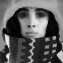
a) Dilation b) Erosion c) Smoothing

d) Gradient e) Laplacian

Figure 46: Examples of gray-level morphological filters.